[Graph] 12/25 간단하게 알아보는 GCN(Graph Convolution Network)

논문 링크: https://arxiv.org/pdf/1609.02907.pdf
참고 자료: https://tkipf.github.io/graph-convolutional-networks/
code: https://github.com/tkipf/pygcn

1. Graph Convolution Network

Graph에 convolultion 기법을 적용한 방법으로 local graph structure를 분석하는 방법론이다. 그로 인해 Spectral graph convolution이라는 의미가 붙는다.
기존에 GCN에 대한 정리 글들을 읽어보았는데 자세히 정리되거나 설명하는 블로그 글이 없어서 이번 기회에 GCN 논문을 제대로 뜯어먹고자 한다.
 

2. Fast Approximated Convolutions on Graph

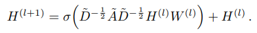
Graph-based neural network model $f(X,A)$을 통해 다음과 같이 layer-wise propagation rule를 고려할 수 있다.

$\hat h = A + I_N$ 으로 loops가 없는, 즉 diagonal element 값이 0인 matrix $A$에 identity matrix $I_N$을 더해줌으로 loops를 추가해 준 모습이다. $\hat D_{ii} = \sum_j \hat A_{ij}$ 으로 loops가 있는 Graph의 Degree를 의미한다. 마지막으로 $W^{(l)}$은 학습 가능한 가중치(weight)이며, $\sigma$는 activation function이다.
참고로 $H^{(0)} = X$이다.
 
2.1. Spectral graph convolutions
Graph에 대해 Spectral convolution을 signal $x \in R^N$ 에 filter $g_{\theta} = diag(\theta)$ 를 곱한 것으로 볼 수 있다.
즉,

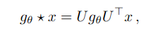
여기서 $U$는 normalized graph Laplacian $L$의 eigenvectors로 다음과 같다.

$L= I_N -D^{-1/2}AD^{-1/2} = UΛU^T$

이를 더 확장시켜 생각해 보면 $g_{\theta}$가 matrix $L$의 eigenvalues라고 볼 수 있다.(즉, $ g_{\theta}(Λ)$)
그러나 위 수식을 바로 적용하기에는 Graph의 크기가 늘어날수록 연산량이 제곱수로 늘어난다는 문제가 있다. 따라서 이를 해결하기 위해서 Chebyshev polynomials $T_k(x)$를 사용한다.

여기서 $\hat Λ = \frac{2}{λ_{max}} Λ - I_N$ 으로 $λ_{max}$은 matrix $L$의 가장 큰 eigenvalue이고 $\theta ^`$은 Chebyshev coefficients이다. 마지막으로 Chebyshev polynomials는 다음과 같이 정의된다.

$T_k(x) = 2xT_{k-1}(x)-T_{k-2}(x)$

초기값 $T_0(x)=1 , T_1(x)=x$이다.
 
이를 앞서 정의했던 signal $x$와 filter $g_{\theta `}$ 에 대한 convolution 정의에 적용하면 아래와 같다.

$\hat L = \frac{2}{λ_{max}}L -I_N$ 이다.
중요점은 위 수식이 K-localized를 의미하는데, 이는 Laplacian의 $K^{th}$-order polynomial로 중심(central) node로부터 최대 K step 거리까지의 node에 의존하기 때문이다. (즉, $K^{th}$-order neighborhood)

• 이를 Graph에 대한 Convolution Neural Network이라는 것이다.

 
 
2.2. Layer-wise linear model
짜증 나게도 위 수식 또한 바로 적용하기에는 local neighborhood structures에 overfitting이 심하고 여전히 연산량이 많다는 문제가 있다. 이 문제들의 경우 아래의 수식을 보면 단번에 이해할 수 있다.

기본적으로 Chebyshev polynomials는 linear formulation이므로 linear coefficient를 알아야 하는데, 위 수식에서 볼 수 있듯이 고려해야 할 parameter가 2개라는 것을 볼 수 있다. 하지만 이로 인해서 연산량이 많아지고 그와 동시에 overfitting 문제가 대두된다.
 
따라서 이를 해결하기 위해서 single parameter을 통해 다음과 같이 수식을 수정한다.

• single parameter: $θ = θ^′_0 = −θ^′_1$

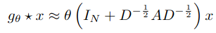
추가적으로 위 operator를 반복적으로 사용했을 때 수치적 불안정성(instabilities)과 exploding/vanishing gradients 문제가 있기 때문에 아래와 같은 renormalization trick을 적용하여 한번 더 수식을 개편한다.
참고로 gradients 문제는 eigenvalues의 range가 $[0,2]$이기 때문이다. (너무나 쉽게 문제가 생길 수 있는 범위)

• renormalization trick: $ I_N+D^{-1/2}AD^{-1/2}  -> \hat D^{-1/2} \hat  A \hat  D^{-1/2}$ 

따라서 최종적으로 수식은 아래와 같다.

 
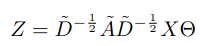
$Z$ 는 convolution signal matrix이다.

 

3. Etc

3.1. Relation to Weisfeiler-Lehman algorithm
Graph structure data에 대해서 잘 분석하는 model은 Graph structure와 Node features 모두 고려하여 node representation을 학습할 수 있어야 한다. nodel label을 할당하는 데 사용되는 연구된 framework는 Weisfeiler-Lehman (WL)이다. 
그래서 WL이 뭐냐고 한다면 이는 아래와 같다.

Graph의 Isomorphism을 판별하는 방법

쉽게 말해서 두 Graph가 동형인지 아닌지를 판별하는 방법이다.
 
그렇다면, 왜 동형인지 아닌지를 구분하는 것이 중요할까?
우리가 하고자 하는 것은 Graph data를 좀 더 분석하기 쉽게 표현(representation) 하는 것이다. 만약 동형이 아니라면, original Graph와 representation Graph가 다르다는 의미이다. 반대로 동형이면, original Graph와 representation Graph가 같다는 의미이다.
좀 더 쉽게 설명하자면, 일대일 대응(=전단사 함수)을 생각하면 된다.

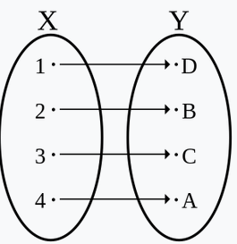
당연하게도 동형사상이 되려면, 사상(mapping)의 형태 또한 일대일 대응이 되어야 한다. 즉, 사상( 또는 함수) $f$ 가 일대일 대응이어야 한다. 따라서 아래와 같은 수식을 적용한다.

이때 $c_{ij}=\sqrt(d_id_j)$로 edge $(v_i,v_j)$에 대한 normalize constant이다. 여기서 $d_i = |N_i|$로 node v_i의 degree를 의미한다. $W^{(l)}$는 weight를 의미한다.
그냥 단순하게 Graph representation에 Symmetrically normalized Laplacian이 적용되었다고 보면 된다.
 
3.2. Node Embedding 
Weisfeiler-Lehman algorithm 분석으로부터, 학습이 되지 않은(Untrained) GCN model이라도 강력한 node feature extractor라는 것을 이해할 수 있다. 왜냐하면, Graph 1개당 단 1개의 representation이 가능하기 때문이다.
 
이를 직관적으로 이해하기 위해 예시로 3-layer GCN model을 아래와 같이 구성할 수 있다

이때 각 weight matrix $W^{(l)}$은 무작위로 초기화된 값을 이용한다.
실험 graph는 undirected & unweighted 로써 34개의 node로 구성되어 있고, 154개의 edge가 있다.
모든 nodes의 label은 4개 중 1개로 되어 있다.

실험 graph는 기본적으로 Karate club network(a)로 구성되어 있으며, 이 초기값에 무작위로 초기화된 $W^{(l)}$를 적용한 것(b)이다.
위 초기값을 바탕으로 300 training iterations, Adam (learning rate: 0.01)을 적용하면 다음과 같은 재미있는 결과가 나온다.

• iterations가 300에 가까울수록 결과가 좋아지고 있음을 볼 수 있다.
• 이와 동시에  GCN model이 classification에 유용한 embedding을 학습하기 위해 Graph structure(및 이후 layer의 Graph structure에서 추출된 feature)를 어떻게 활용할 수 있는지에 대한 통찰력을 제공한다. 

 
 
3.3. Experiments on Model Depth
위에서 정의되었던 수식(아래 참고)을 이용하여 layer를 구성하였을 때, layer의 깊이(depth)에 따른 모델 성능 평가이다.

residual 적용

결과는 아래와 같다.

• 일반적으로 많은 graph nerual network에서 layer를 쌓을 때 깊이를 2개 정도로 하게 되는데 아무래도 위와 같은 결과 때문이지 않을까 한다.
• training set에 대해서는 정확성(Accuracy)이 높지만 testing set에 대해서는 layer가 2 이후로 크게 차이가 없거나 값이 떨어지는 것을 볼 수가 있다. 이는 layer가 깊은 경우 overfitting이 발생했다고 해석할 수 있다. 

4. Code

4.1. pre-processing
아래와 같은 수식을 data에 적용하여 pre-processing한다.

def load_data(path="../data/cora/", dataset="cora"):
    """Load citation network dataset (cora only for now)"""
    print('Loading {} dataset...'.format(dataset))

    idx_features_labels = np.genfromtxt("{}{}.content".format(path, dataset),
                                        dtype=np.dtype(str))
    features = sp.csr_matrix(idx_features_labels[:, 1:-1], dtype=np.float32)
    labels = encode_onehot(idx_features_labels[:, -1])

    # build graph
    idx = np.array(idx_features_labels[:, 0], dtype=np.int32)
    idx_map = {j: i for i, j in enumerate(idx)}
    edges_unordered = np.genfromtxt("{}{}.cites".format(path, dataset),
                                    dtype=np.int32)
    edges = np.array(list(map(idx_map.get, edges_unordered.flatten())),
                     dtype=np.int32).reshape(edges_unordered.shape)
    adj = sp.coo_matrix((np.ones(edges.shape[0]), (edges[:, 0], edges[:, 1])),
                        shape=(labels.shape[0], labels.shape[0]),
                        dtype=np.float32)

    # build symmetric adjacency matrix
    adj = adj + adj.T.multiply(adj.T > adj) - adj.multiply(adj.T > adj)

    features = normalize(features)
    adj = normalize(adj + sp.eye(adj.shape[0]))

    idx_train = range(140)
    idx_val = range(200, 500)
    idx_test = range(500, 1500)

    features = torch.FloatTensor(np.array(features.todense()))
    labels = torch.LongTensor(np.where(labels)[1])
    adj = sparse_mx_to_torch_sparse_tensor(adj)

    idx_train = torch.LongTensor(idx_train)
    idx_val = torch.LongTensor(idx_val)
    idx_test = torch.LongTensor(idx_test)

    return adj, features, labels, idx_train, idx_val, idx_test


def normalize(mx):
    """Row-normalize sparse matrix"""
    rowsum = np.array(mx.sum(1))
    r_inv = np.power(rowsum, -1).flatten()
    r_inv[np.isinf(r_inv)] = 0.
    r_mat_inv = sp.diags(r_inv)
    mx = r_mat_inv.dot(mx)
    return mx

 
 
4.2. Layer
아래의 수식을 구성하는 코드이다.

import math

import torch

from torch.nn.parameter import Parameter
from torch.nn.modules.module import Module


class GraphConvolution(Module):
    """
    Simple GCN layer, similar to https://arxiv.org/abs/1609.02907
    """

    def __init__(self, in_features, out_features, bias=True):
        super(GraphConvolution, self).__init__()
        self.in_features = in_features
        self.out_features = out_features
        self.weight = Parameter(torch.FloatTensor(in_features, out_features))
        if bias:
            self.bias = Parameter(torch.FloatTensor(out_features))
        else:
            self.register_parameter('bias', None)
        self.reset_parameters()

    def reset_parameters(self):
        stdv = 1. / math.sqrt(self.weight.size(1))
        self.weight.data.uniform_(-stdv, stdv)
        if self.bias is not None:
            self.bias.data.uniform_(-stdv, stdv)

    def forward(self, input, adj):
        support = torch.mm(input, self.weight)
        output = torch.spmm(adj, support)
        if self.bias is not None:
            return output + self.bias
        else:
            return output

    def __repr__(self):
        return self.__class__.__name__ + ' (' \
               + str(self.in_features) + ' -> ' \
               + str(self.out_features) + ')'

 
4.3. Layer 쌓기
그런 다음 layer를 2개 쌓아 graph convolution nerual network를 구성하는 모습이다. 

import torch.nn as nn
import torch.nn.functional as F
from pygcn.layers import GraphConvolution


class GCN(nn.Module):
    def __init__(self, nfeat, nhid, nclass, dropout):
        super(GCN, self).__init__()

        self.gc1 = GraphConvolution(nfeat, nhid)
        self.gc2 = GraphConvolution(nhid, nclass)
        self.dropout = dropout

    def forward(self, x, adj):
        x = F.relu(self.gc1(x, adj))
        x = F.dropout(x, self.dropout, training=self.training)
        x = self.gc2(x, adj)
        return F.log_softmax(x, dim=1)