[Graph] 12/10 간단하게 알아보는 GAT(Graph Attention Network)

paper

Graph Attention Networks

연구의 필요성

CNN 은 image classification ,segmentation 및 machine translation 에 좋은 성능을 보여줌.

이러한 data는 grid와 같은 구조(structure)를 가짐.

이러한 모델 구조(architectures)는 학습 가능한 local filter를 모든 입력 위치에 적용하여 효과적으로 재사용

그러나 많은 흥미로운 작업에는 grid와 같은 구조(structure)로 표현될 수 없는 데이터가 포함되며, 대신에 그것은 불규칙한 영역에 있음.

• e.g. 3D meshes, social networks, telecommunication networks,…
• 위 예시들은 모두 graph form으로 나타낼 수 있음.

선행 연구들

임의로 구성된(structed) graph를 다루기 위한 시도들은 많이 있었음.

• RNN(Recursive Nerual Networks) 통한 방법
• GNN을 통한 방법

GNN의 경우 다음과 같이 설명 가능

• node states가 동일(equilibrium)할 때 까지 반복함.
• DNN을 통해 state에 따라 각 node에 대한 출력 생성

최근 GNN 연구들은 convolution을 일반화 하는데 집중하고 있음.

• Spectral approach (e.g. Graph Convolution Network)
  
  • graph를 spectral로 표현, node 분류에 성공적
  • 이러한 방법은 Laplacian eigenbasis에 연관 learned filter
    • Graph 구조(structure)에 의존적
    • 학습된 Graph와 다른 구조에는 적용 불가능. = 따로 학습 시켜야 함
• Non-spectral approach (GraphSAGE)
  
  • Convolutions을 graph에 직접 적용.
    • 공간적으로 가까운 이웃 그룹에서 작동
    • 다양한 크기의 이웃(neighborhood)과 함께 작동
    • CNN의 가중치 공유 속성을 유지하는 연산자를 정의하는 것에 대해 문제를 다룸

Attention mechanism

• 다양한 size를 가지는 input에 대해서 다룰 수 있음
• 입력 중 가장 관련성이 높은 부분에 집중
• machine translation task에서 SOTA를 차지

제안 방법

GAT archtecture

1. Graph Attentional Layer
2. 학습 가능한 linear transform
3. Attention mechanism
4. Attention normalize
5. Multi-head attention

1. Graph Attention Layer

N을 node 개수, F를 각 노드의 feature 개수라고 하면 input과 output을 다음과 같이 나타낼 수 있다.

input: $ h = [\overline h_1, \overline h_2 ,..., \overline h_N], \overline h_1 \in R^F $

output: $ h^′ = [\overline h^′_1, \overline h^′_2 ,..., \overline h^′_N], \overline h^′_1 \in R^{F^′} $

 

2. 학습 가능한 linear transform

입력 특징을 더 높은 수준의 특징(higher-level features)으로 변환하기 위해 학습 가능한 linear transform이 하나 이상 필요

                = regression을 생각하면 됨.

                = 독립(indenpendent)조합으로 이루어진 새로운 function

                = higher-level features

 

이를 $W \in R^{F^′ \times F}$ 로 표현, 모든 node에 대해서 적용

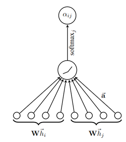
3. Attention mechanism

앞서 계산된 node에 대해서 attention 적용

Attention coefficient를 $a$라고 표현

$$a: R^{F^′} \times R^{F^′}$$    

node i 입장에서 바라본 node j의 중요도(importance)를 의미.

model은 모든 node가 다른 모든 node에 참여하도록 허용하여 모든 구조적(structural) 정보를 삭제

                = 다른 graph에 대해서도 적용 가능

                = 귀납적(inductive) 방법

Masked attention을 수행하여 self attention mechanism에 graph structure를 주입

node i $ \in N_i$ 에 대해서만 $e_{ij}$를 계산, 여기서 $N_i$는 graph 에서 node i의 일부 이웃

4. Attention normalize

다른 node와 쉽게 비교를 위해서 softmax function을 통해 normalize

softmax

실험적으로 LeakyReLU nonlinearity를 사용

apply LeakyReLU

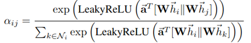
참고로 ||은 concatenation operator임 = (torch.cat)

                => || operator은 일대일(injective function)

                = 비교 결과(attention 결과)가 중복 없음

                = 모든 결과가 서로 다름

                = node 중요도(importance)가 다 다름

최종적으로 output은 다음과 같음

Attention

아래 이미지는 concat operator가 적용된 graph

5. Multi-head attention

stabilize을 위해서 multi-head attention 기법 적용

앞서 언급된 최종 output 수식에서 ||을 사용하기만 하면 됨

Multi-head Attention

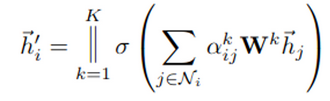
즉, 모든 node의 attention들을 합친 것

                = node 한 개당 본인 포함 N개에 해당하는 attenction coeff 있음

                = 모든 node에 대해서 concat 하므로 $\overline h^′_i \in R^{F^′} \times R^{F^′}$

 

하지만 이로 인해(concat 연산자로 인해) network는 더 이상 민감(sensible)하지 않음

                = 한 grpah 내에서 node i 와 비교된 node j 가 각각 다름

                = node i 에 대한 edge 연결이 다 다름 

                = attention coeff 결과가 다 다름 

                = concate operator는 이를 반영하지 못함

                = 추가적인 가중치 또는 normalize 필요

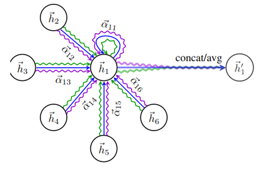
따라서 아래와 같이 Averaging 적용

Averaging

아래 이미지는 Multi head attention과 Averaging 이 적용된 Graph

간단한 코드 구현 (본 코드는 mutli-head 부분은 생략 ( Averaging 생략 ))

def mlp(input_dim, mlp_dims, last_relu=False):
    layers = []
    mlp_dims = [input_dim] + mlp_dims
    for i in range(len(mlp_dims) - 1):
        layers.append(nn.Linear(mlp_dims[i], mlp_dims[i + 1]))
        if i != len(mlp_dims) - 2 or last_relu:
            layers.append(nn.ReLU())
    net = nn.Sequential(*layers)
    return net

class GraphAttentionLayer(nn.Module):

    def __init__(self, in_features, out_features, dropout=0.,training = True):
        super(GraphAttentionLayer, self).__init__()
        self.in_features = in_features
        self.out_features = out_features
        self.training = training
        self.dropout = dropout
        self.act = nn.ReLU()
        self.w_a = mlp(2 * self.in_features, [2 * self.in_features, 1], last_relu=False)
        self.weight = Parameter(torch.FloatTensor(2*in_features, out_features))
        self.leakyrelu = nn.LeakyReLU(negative_slope=0.04)

    def reset_parameters(self):
        torch.nn.init.xavier_uniform_(self.weight)

    def forward(self, input, adj):

        assert len(input.shape) == 3
        assert len(adj.shape) == 3
        input = F.dropout(input, self.dropout, self.training)

        A = self.compute_similarity_matrix(input)
        e = self.leakyrelu(A) 
        
        zero_vec = -9e15 * torch.ones_like(e)
        attention = torch.where(adj > 0, e, zero_vec)
        attention = nn.functional.softmax(attention, dim=2)
        next_H = torch.matmul(attention, input)
        
        return next_H, attention[0, 0, :].data.cpu().numpy()

    def compute_similarity_matrix(self, X):
 
        indices = [pair for pair in itertools.product(list(range(X.size(1))), repeat=2)]
        selected_features = torch.index_select(X, dim=1, index=torch.LongTensor(indices).reshape(-1))
        pairwise_features = selected_features.reshape((-1, X.size(1) * X.size(1), X.size(2) * 2))
        A = self.w_a(pairwise_features).reshape(-1, X.size(1), X.size(1))

        return A